本节主要介绍了多层感知机、K-折交叉验证、欠拟合与过拟合以及权重衰退
多层感知机
我们可以通过在网络中加入一个或多个隐藏层来克服线性模型的限制, 使其能处理更普遍的函数关系类型。
要做到这一点,最简单的方法是将许多全连接层堆叠在一起,每一层都输出到上面的层,直到生成最后的输出
我们可以把前$L−1$层看作表示,把最后一层看作线性预测器
这种架构通常称为多层感知机(multilayer perceptron),通常缩写为MLP
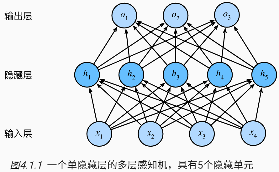
这个多层感知机有4个输入,3个输出,其隐藏层包含5个隐藏单元
输入层不涉及任何计算,因此使用此网络产生输出只需要实现隐藏层和输出层的计算,因此,这个多层感知机中的层数为2
注意,这两个层都是全连接的,每个输入都会影响隐藏层中的每个神经元, 而隐藏层中的每个神经元又会影响输出层中的每个神经元
多层感知机在输出层和输入层之间增加一个或多个全连接隐藏层,并通过激活函数转换隐藏层的输出
- 常用的激活函数包括ReLU函数、sigmoid函数和tanh函数
多层感知机的简洁实现
1 | import torch |
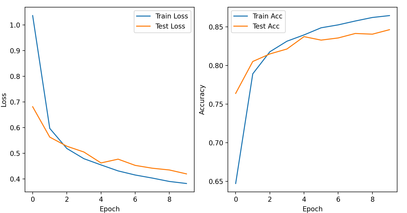
结果如下:
1 | Epoch [1/10], Train Loss: 1.0367, Train Acc: 64.71%, Test Loss: 0.6816, Test Acc: 76.38% |
with torch.no_grad()的理解:【pytorch系列】 with torch.no_grad():用法详解_大黑山修道的博客-CSDN博客
K-折交叉验证
非大数据集上通常使用k-折交叉验证
训练数据集:训练模型参数
验证数据集:选择模型超参数
K-折交叉验证的算法:
- 将训练数据分割成K块
For i = 1,…,K
- 使用第i块作为验证数据集,其余的k-1块作为训练数据集
报告K个验证集误差的平均
常用K=5或10
例如:若K=3
| | 块1 | 块2 | 块3 |
| —— | ——- | ——- | ——- |
| i=1 | val | train | train |
| i=2 | train | val | train |
| i=3 | train | train | val |
欠拟合与过拟合
模型容量:
- 拟合各种函数的能力
- 低容量的模型难以拟合训练数据
- 高容量的模型可以记住所有的训练数据
过拟合与欠拟合
| | 数据:简单 | 数据:复杂 |
| ———————— | ——————— | ——————— |
| 模型容量:低 | 正常 | 欠拟合 |
| 模型容量:高 | 过拟合 | 正常 |- 过拟合:在训练集上表现好,但是在测试集上效果差
- 欠拟合(高偏差):模型拟合不够,在训练集上表现效果差,没有充分的利用数据,预测的准确度低
- 偏差:反映的是模型在样本上的输出与真实值之间的误差,即模型本身的精确度
- 方差:反映的是模型每一次输出结果与模型输出期望之间的误差,即模型的稳定性
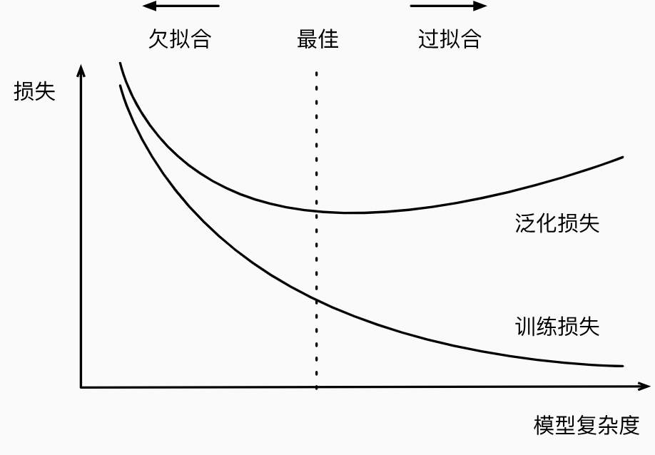
模型复杂度对欠拟合和过拟合的影响
如何防止过拟合与欠拟合:
- 防止过拟合方法:
- 补充数据集
- 减少模型参数
- Dropout
- Earlystopping
- 正则化或稀疏化
- 防止欠拟合方法
- 加大模型参数
- 减少正则化参数
- 更充分的训练
- 防止过拟合方法:
权重衰退($L_2$正则化)
在训练参数化机器学习模型时, 权重衰减(weight decay)是最广泛使用的正则化的技术之一, 它通常也被称为$L_2$正则化
使用均方范数作为硬性限制:
通过限制参数值的选择范围来控制模型容量
通常不限制偏移b
小的$\theta$意味着更强的正则项
使用均方范数作为柔性限制
对于每一个$\theta$,都可以找到$\lambda$使得之前的目标函数等价于:
超参数$\lambda$控制了正则项的重要程度
- $\lambda=0$:正则项无作用
- $\lambda\rightarrow \infty$:意味着$\theta\rightarrow0$,$w\rightarrow0$
参数更新法则:
计算梯度:
时间t更新参数:
通常$\eta\lambda<1$,在深度学习中通常叫做权重衰退