本节主要介绍了回归问题与分类问题
线性回归从零开始实现
1 | import random |
结果如下:
1 | features: tensor([-1.7930, -0.8309]) |
线性回归的简洁实现
1 | import numpy as np |
结果如下:
1 | [tensor([[-0.8065, 0.9427], |
next理解参考:Python next() 函数 (w3school.com.cn)
波斯顿房价预测实现
1.网络搭建与训练
1 | import torch |
2.模型测试与评估
1 | import torch |
softmax回归
1.softmax函数
softmax函数能够将未规范化的预测变换为非负数并且总和为1,同时让模型保持 可导的性质
其中$z_i$为第$i$个节点的输出值,C为输出节点的个数,即分类的类别个数
2.损失函数
对于任何标签$y$和模型预测$\hat{y}$(回归模型经过softmax函数后的预测概率值),损失函数为:
该损失函数通常被称为交叉熵损失
由于$y$是一个长度为$q$的独热编码向量,所以除一个项以外的所有项$j$都消失了
由于所有$\hat{y}$都是预测的概率,所以它们的对数永远不会大于0
3.图像分类数据集Fashion-mnist
Fashion-MNIST由10个类别的图像组成, 每个类别由训练数据集(train dataset)中的6000张图像和测试数据集(test dataset)中的1000张图像组成
因此,训练集和测试集分别包含60000和10000张图像
测试数据集不会用于训练,只用于评估模型性能
每个输入图像的高度和宽度均为28像素。 数据集由灰度图像组成,其通道数为1
将高度$h$像素、宽度$w$像素图像的形状记为$h\times w$或$(h,w)$
transforms.ToTensor() 的作用是将 PIL 图像或 NumPy 数组转换为一个张量(Tensor)格式,并将其归一化为值在 [0,1] 之间的浮点数
torchvision.datasets.FashionMNIST函数返回的是一个Dataset对象,而不是一个Tensor对象。因此,不能通过调用shape属性来获取数据集的大小和形状1
2
3
4
5
6
7
8
9
10
11
12
13
14
15
16
17
18
19
20
21
22
23
24
25
26
27
28
29
30
31
32
33
34
35
36
37
38
39
40
41
42
43
44
45
46
47
48
49
50
51
52
53
54
55
56
57
58
59
60
61
62
63
64
65
66
67
68
69
70
71
72
73
74
75
76
77
78
79
80import torch
import torchvision
from torch.utils import data
from torchvision import transforms
import time
import numpy as np
import matplotlib.pyplot as plt
#定义一个计时器
class Timer: #@save
"""记录多次运行时间"""
def __init__(self):
self.times = []
self.start()
def start(self):
"""启动计时器"""
self.tik = time.time()
def stop(self):
"""停止计时器并将时间记录在列表中"""
self.times.append(time.time() - self.tik)
return self.times[-1]
def avg(self):
"""返回平均时间"""
return sum(self.times) / len(self.times)
def sum(self):
"""返回时间总和"""
return sum(self.times)
def cumsum(self):
"""返回累计时间"""
return np.array(self.times).cumsum().tolist()
#读取数据集
trans = transforms.ToTensor() #通过ToTensor实例将图像数据从PIL类型变换成32位浮点数格式
mnist_train = torchvision.datasets.FashionMNIST(
root="D:\App_Data_File\VScode_Project\Python\Pytorch\dataset\Fashion-MNIST", train=True, transform=trans, download=True)
mnist_test = torchvision.datasets.FashionMNIST(
root="D:\App_Data_File\VScode_Project\Python\Pytorch\dataset\Fashion-MNIST", train=False, transform=trans, download=True)
#获取mnist_train中的第一个样本,即 mnist_train[0]。
#这个样本包含一个图像数据和一个标签
#使用一个元组来将它们分别赋值给image和label变量
#最后,输出image的形状,以查看它的维度信息
sample = mnist_train[0] # 获取第一个样本
image, label = sample
print(image.shape) # 输出训练集第一个图像数据的形状
#Fashion-MNIST中包含的10个类别
#分别为t-shirt(T恤)、trouser(裤子)、pullover(套衫)、dress(连衣裙)、coat(外套)
#sandal(凉鞋)、shirt(衬衫)、sneaker(运动鞋)、bag(包)和ankle boot(短靴)
#以下函数用于在数字标签索引及其文本名称之间进行转换。
def get_fashion_mnist_labels(labels): #@save
"""返回Fashion-MNIST数据集的文本标签"""
text_labels = ['t-shirt', 'trouser', 'pullover', 'dress', 'coat',
'sandal', 'shirt', 'sneaker', 'bag', 'ankle boot']
return text_labels[labels]
#画出数据集中前20个训练集的图像
# fig, axs = plt.subplots(4, 5, figsize=(10, 8))
# for i in range(20):
# image, label = mnist_train[i]
# row, col = divmod(i, 5)
# axs[row, col].imshow(image.squeeze(), cmap='CMRmap')
# axs[row, col].set_title(f'Label: {get_fashion_mnist_labels(label)}')
# axs[row, col].axis('off')
# plt.show()
##读取小批量数据集
batch_size = 256
train_iter = data.DataLoader(mnist_train, batch_size, shuffle=True)
#查看读取数据集所需要的时间
timer = Timer()
for X, y in train_iter:
continue
print(f'{timer.stop():.2f} sec')结果如下:
1
2
torch.Size([1, 28, 28])
2.00 sec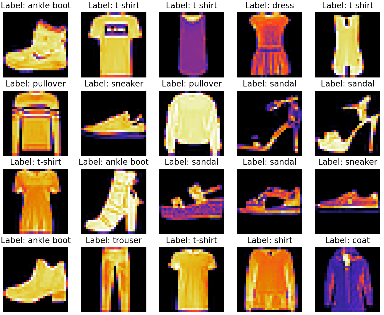
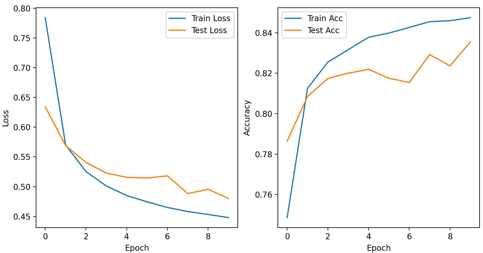
softmax回归的简洁实现
1 | import torch |
结果如下:
1 | Epoch [1/10], Train Loss: 0.7841, Train Acc: 74.86%, Test Loss: 0.6342, Test Acc: 78.64% |
手写数字集的识别
1.数据集处理与模型训练
1 | import torch |
2.网络搭建
1 | import torch |
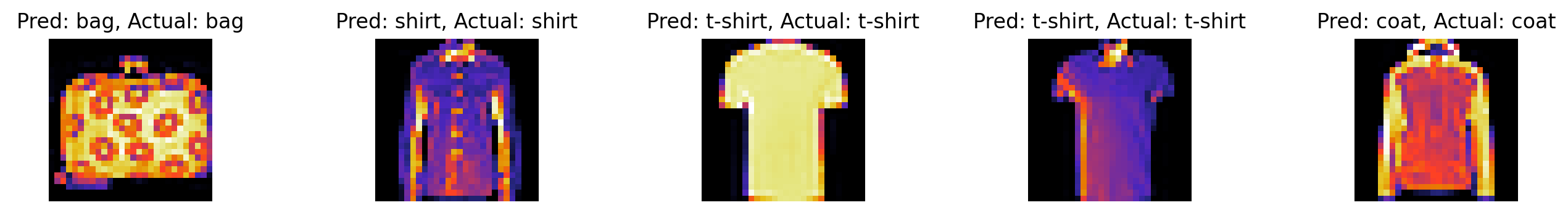
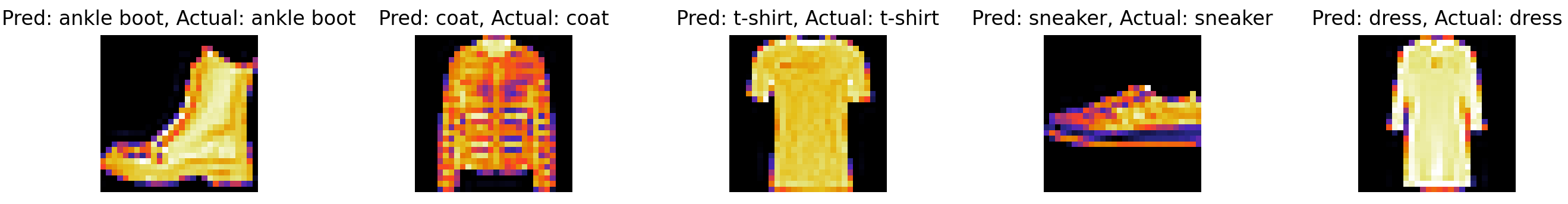
3.模型测试与评估
1 | import torch |
交叉熵损失函数
- torch.nn.CrossEntropyLoss()实际上是LogSoftmax与NLLLoss函数的叠加
- 则在使用torch.nn.CrossEntropyLoss()时,不需要在网络输出中经过softmax层
- torch.nn.CrossEntropyLoss()的输入可以是独热编码,也可以是直接是标签分类值
- pytorch 多分类中的损失函数 - 宋桓公 - 博客园 (cnblogs.com)
- torch.nn.CrossEntropyLoss() 参数、计算过程以及及输入Tensor形状 - 知乎 (zhihu.com)