1
2
3
4
5
6
7
8
9
10
11
12
13
14
15
16
17
18
19
20
21
22
23
24
25
26
27
28
29
30
31
32
33
34
35
36
37
38
39
40
41
42
43
44
45
46
47
48
49
50
51
52
53
54
55
56
57
58
59
60
61
62
63
64
65
66
67
68
69
70
71
72
73
74
75
76
77
78
79
80
81
82
83
84
85
86
87
88
89
90
91
92
93
94
95
96
97
98
99
100
101
| import tensorflow as tf
import numpy as np
import matplotlib.pyplot as plt
import pandas as pd
import matplotlib as mpl
TRAIN_URL = "http://download.tensorflow.org/data/iris_training.csv"
train_path = tf.keras.utils.get_file("iris_train.csv",TRAIN_URL,cache_dir="D:\App_Data_File\Anaconda_data\jupyter\TensorFlow")
TRAIN_URL = "http://download.tensorflow.org/data/iris_test.csv"
test_path = tf.keras.utils.get_file("iris_test.csv",TRAIN_URL,cache_dir="D:\App_Data_File\Anaconda_data\jupyter\TensorFlow")
df_iris_train=pd.read_csv(train_path,header=0)
df_iris_test=pd.read_csv(test_path,header=0)
iris_train=np.array(df_iris_train)
iris_test=np.array(df_iris_test)
train_x=iris_train[:,0:2]
test_x=iris_test[:,0:2]
train_y=iris_train[:,4]
test_y=iris_test[:,4]
x_train=train_x[train_y<2]
y_train=train_y[train_y<2]
x_test=test_x[test_y<2]
y_test=test_y[test_y<2]
num_train=len(x_train)
num_test=len(x_test)
cm_pt=mpl.colors.ListedColormap(["blue","red"])
x_train=x_train-np.mean(x_train,axis=0)
x_test=x_test-np.mean(x_test,axis=0)
x0_train=np.ones(num_train).reshape(-1,1)
X_train=tf.cast(tf.concat((x0_train,x_train),axis=1),tf.float32)
Y_train=y_train.reshape(-1,1)
x0_test=np.ones(num_test).reshape(-1,1)
X_test=tf.cast(tf.concat((x0_test,x_test),axis=1),tf.float32)
Y_test=y_test.reshape(-1,1)
learn_rate=0.2
iter=120
display_step=30
np.random.seed(612)
W=tf.Variable(np.random.randn(3,1),dtype=tf.float32)
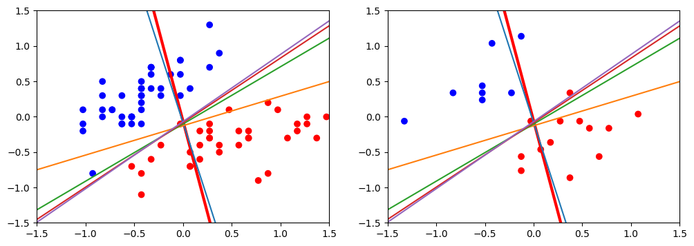
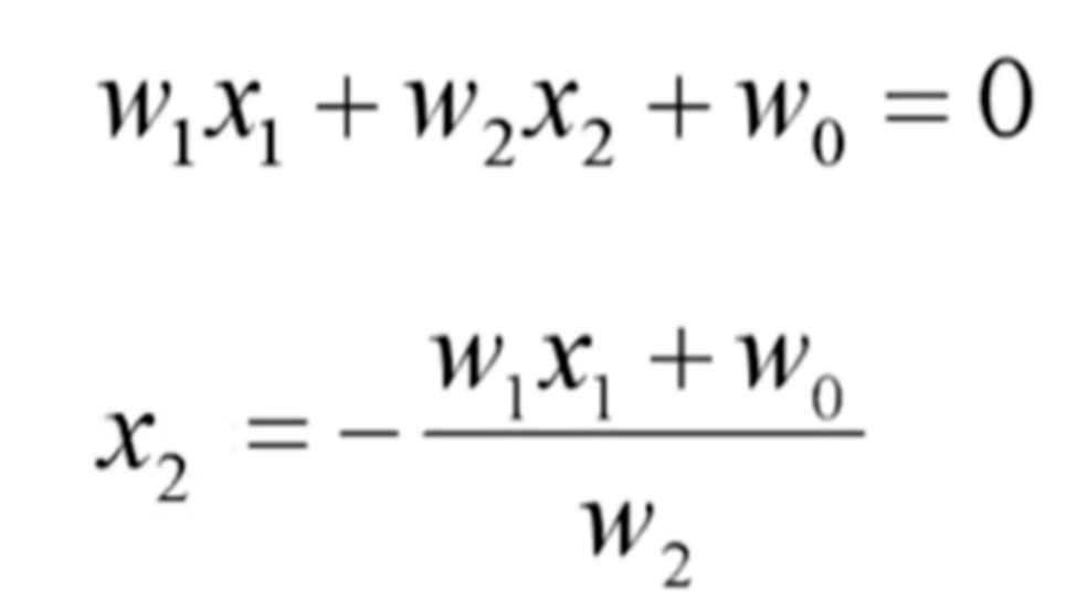
x_=[-1.5,1.5]
y_=-(W[0]+W[1]*x_)/W[2]
plt.figure(figsize=(12,4))
plt.subplot(121)
plt.scatter(x_train[:,0],x_train[:,1],c=y_train,cmap=cm_pt)
plt.plot(x_,y_,color="red",linewidth=3)
plt.xlim(-1.5,1.5)
plt.ylim(-1.5,1.5)
plt.subplot(122)
plt.scatter(x_test[:,0],x_test[:,1],c=y_test,cmap=cm_pt)
plt.plot(x_,y_,color="red",linewidth=3)
plt.xlim(-1.5,1.5)
plt.ylim(-1.5,1.5)
ce_train=[]
acc_train=[]
ce_test=[]
acc_test=[]
for i in range(0,iter+1):
with tf.GradientTape() as tape:
PRED_train=1/(1+tf.exp(-tf.matmul(X_train,W)))
Loss_train=-tf.reduce_mean(Y_train*tf.math.log(PRED_train)+(1-Y_train)*tf.math.log(1-PRED_train))
PRED_test=1/(1+tf.exp(-tf.matmul(X_test,W)))
Loss_test=-tf.reduce_mean(Y_test*tf.math.log(PRED_test)+(1-Y_test)*tf.math.log(1-PRED_test))
Accuracy_train=tf.reduce_mean(tf.cast(tf.equal(tf.where(PRED_train<0.5,0,1),Y_train),tf.float32))
Accuracy_test=tf.reduce_mean(tf.cast(tf.equal(tf.where(PRED_test<0.5,0,1),Y_test),tf.float32))
ce_train.append(Loss_train)
acc_train.append(Accuracy_train)
ce_test.append(Loss_test)
acc_test.append(Accuracy_test)
dL_dW=tape.gradient(Loss_train,W)
W.assign_sub(learn_rate*dL_dW)
if i % display_step==0:
print("i:%i\tTrain Loss:%f\tAccuracy Train:%f\t\tTest Loss:%f\tAccuracy Test:%f" % (i,Loss_train,Accuracy_train,Loss_test,Accuracy_test))
y_=-(W[0]+W[1]*x_)/W[2]
plt.subplot(121)
plt.plot(x_,y_)
plt.subplot(122)
plt.plot(x_,y_)
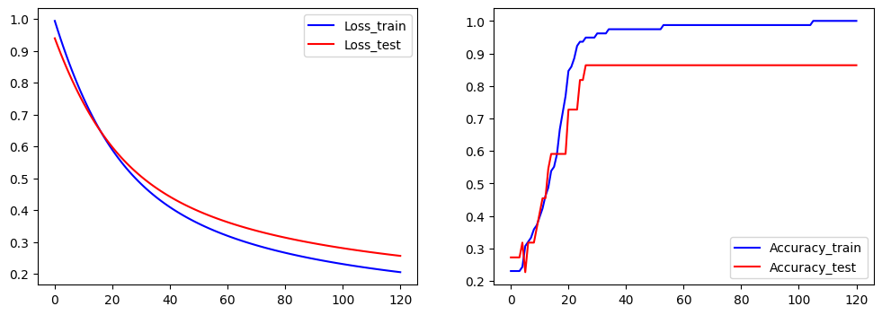
plt.figure(figsize=(12,4))
plt.subplot(121)
plt.plot(ce_train,color="blue",label="Loss_train")
plt.plot(ce_test,color="red",label="Loss_test")
plt.legend()
plt.subplot(122)
plt.plot(acc_train,color="blue",label="Accuracy_train")
plt.plot(acc_test,color="red",label="Accuracy_test")
plt.legend()
|