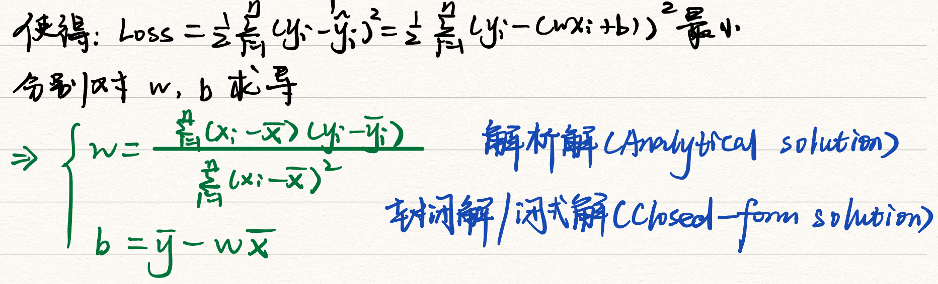
本节主要介绍了如何通过解析法与梯度下降法求解线性回归问题。

解析法实现一元线性回归

加载样本数据：x、y
学习模型：计算w、b
预测：y_pred=w*x_test+b

1.纯Python实现

#加载样本数据：x、y
x=[137.97,104.50,100.00,124.32,79.20,99.00,124.00,114.00,106.69,138.05,53.75,46.91,68.00,63.02,81.26,86.21]
y=[145.00,110.00,93.00,116.00,65.32,104.00,118.00,91.00,62.00,133.00,51.00,45.00,78.50,69.65,75.69,95.30]
#学习模型：计算w、b
x_mean=sum(x)/len(x)
y_mean=sum(y)/len(y)
sumXY=0.0
sumX=0.0
for i in range(len(x)):
    sumXY+=(x[i]-x_mean)*(y[i]-y_mean)
    sumX+=pow((x[i]-x_mean),2)
w=sumXY/sumX
b=y_mean-w*x_mean
print("w:",w)
print("b:",b)
#预测房价
x_test=[128.15,45.00,141.43,106.27,99.00,53.84,85.36,70.00]
for i in range(len(x_test)):
    print("The Y of",x_test[i],'is:',w*x_test[i]+b)

结果如下：

w: 0.8945605120044221
b: 5.410840339418002
The Y of 128.15 is: 120.0487699527847
The Y of 45.0 is: 45.66606337961699
The Y of 141.43 is: 131.92853355220342
The Y of 106.27 is: 100.47578595012793
The Y of 99.0 is: 93.97233102785579
The Y of 53.84 is: 53.57397830573609
The Y of 85.36 is: 81.77052564411547
The Y of 70.0 is: 68.03007617972756

2.NumPy实现

import numpy as np
#加载样本数据：x、y
x=np.array([137.97,104.50,100.00,124.32,79.20,99.00,124.00,114.00,106.69,138.05,53.75,46.91,68.00,63.02,81.26,86.21])
y=np.array([145.00,110.00,93.00,116.00,65.32,104.00,118.00,91.00,62.00,133.00,51.00,45.00,78.50,69.65,75.69,95.30])
#学习模型
x_mean=np.mean(x)
y_mean=np.mean(y)
sumXY=np.sum((x-x_mean)*(y-y_mean))
sumX=np.sum((x-x_mean)**2)
w=sumXY/sumX
b=y_mean-w*x_mean
print("w:",w)
print("b:",b)
#预测房价
x_test=np.array([128.15,45.00,141.43,106.27,99.00,53.84,85.36,70.00])
Y=w*x_test+b
print("The Y is:",Y)

结果如下：

w: 0.894560512004422
b: 5.410840339418002
The Y is: [120.04876995  45.66606338 131.92853355 100.47578595  93.97233103
  53.57397831  81.77052564  68.03007618]

3.TensorFlow实现

import tensorflow as tf
#加载样本数据：x、y
x=tf.constant([137.97,104.50,100.00,124.32,79.20,99.00,124.00,114.00,106.69,138.05,53.75,46.91,68.00,63.02,81.26,86.21])
y=tf.constant([145.00,110.00,93.00,116.00,65.32,104.00,118.00,91.00,62.00,133.00,51.00,45.00,78.50,69.65,75.69,95.30])
#学习模型
x_mean=tf.reduce_mean(x)
y_mean=tf.reduce_mean(y)
sumXY=tf.reduce_sum((x-x_mean)*(y-y_mean))
sumX=tf.reduce_sum((x-x_mean)**2)
w=sumXY/sumX
b=y_mean-w*x_mean
print("w:",w.numpy())
print("b:",b.numpy())
#预测房价
x_test=tf.constant([128.15,45.00,141.43,106.27,99.00,53.84,85.36,70.00])
Y=w*x_test+b
print("The Y is:",Y.numpy())

结果如下：

w: 0.8945604
b: 5.4108505
The Y is: [120.04876   45.66607  131.92853  100.475784  93.97233   53.573982
  81.77052   68.030075]

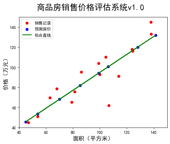
4.数据和模型可视化

#导入库
import numpy as np
import tensorflow as tf
import matplotlib.pyplot as plt
#加载数据样本
x=tf.constant([137.97,104.50,100.00,124.32,79.20,99.00,124.00,114.00,106.69,138.05,53.75,46.91,68.00,63.02,81.26,86.21])
y=tf.constant([145.00,110.00,93.00,116.00,65.32,104.00,118.00,91.00,62.00,133.00,51.00,45.00,78.50,69.65,75.69,95.30])
#学习模型
x_mean=tf.reduce_mean(x)
y_mean=tf.reduce_mean(y)
sumXY=tf.reduce_sum((x-x_mean)*(y-y_mean))
sumX=tf.reduce_sum((x-x_mean)**2)
w=sumXY/sumX
b=y_mean-w*x_mean
print("线性模型：y={}*x+{}".format(w.numpy(),b.numpy()))
#预测房价
x_test=np.array([128.15,45.00,141.43,106.27,99.00,53.84,85.36,70.00])
Y=(w*x_test+b).numpy()
print("面积\t房价")
for i in range(len(x_test)):
    print(x_test[i],"\t",round(Y[i],2)) #round()四舍五入保留小数
#可视化
plt.figure(num="一维线性回归数据可视化")
plt.rcParams["font.sans-serif"]="SimHei"
plt.rcParams["axes.unicode_minus"]=False
plt.scatter(x,y,color="red",label="销售记录")
plt.scatter(x_test,Y,color="blue",label="预测房价")
plt.plot(x_test,Y,color="green",label="拟合直线",linewidth=2)
plt.xlabel("面积（平方米）",fontsize=14)
plt.ylabel("价格（万元）",fontsize=14)
plt.xlim(40,150)
plt.ylim(40,150)
plt.suptitle("商品房销售价格评估系统v1.0",fontsize=20)
plt.legend(loc=2)
plt.show()

结果如下：

线性模型：y=0.8945603966712952*x+5.410850524902344
面积    房价
128.15      120.05
45.0      45.67
141.43      131.93
106.27      100.48
99.0      93.97
53.84      53.57
85.36      81.77
70.0      68.03

解析法实现多元线性回归

加载样本数据
数据处理：将输入的数据转化为模型要求的形式
学习模型：计算W
预测：Y=X@W

import numpy as np
#加载样本数据
x1=np.array([137.97,104.50,100.00,124.32,79.20,99.00,124.00,114.00,106.69,138.05,53.75,46.91,68.00,63.02,81.26,86.21])
x2=np.array([3,2,2,3,1,2,3,2,2,3,1,1,1,1,2,2])
y=np.array([145.00,110.00,93.00,116.00,65.32,104.00,118.00,91.00,62.00,133.00,51.00,45.00,78.50,69.65,75.69,95.30])
#数据处理：将输入的数据转化为模型要求的形式
#1.X：16*3
x0=np.ones(len(x1))
X=np.stack([x0,x1,x2],axis=1)
print("The X is:\n",X)
#2.Y：16*1
Y=y.reshape(-1,1)#-1表示根据数量自动匹配行的长度
print("The Y is:\n",Y)
#求解模型参数W
#1.计算X'
Xt=np.transpose(X)
#2.计算(X'X)-1
XtX_1=np.linalg.inv(np.matmul(Xt,X))
#3.计算(X'X)-1X'
XtX_1_Xt=np.matmul(XtX_1,Xt)
#4.计算W=(X'X)-1X'Y
W=np.matmul(XtX_1_Xt,Y)
print("The W is:\n",W)
#转置W方便打印显示
W=W.reshape(-1)
print("多元线性回归方程：Y={}*x1+{}*x2+{}".format(W[1],W[2],W[0]))
#预测房价
print("请输入房屋面积和房间数，预测房屋销售价格：")
x1_test=float(input("商品房面积："))
x2_test=float(input("房间数："))
Y_pred=W[1]*x1_test+W[2]*x2_test+W[0]
print("预测价格：",round(Y_pred,2),"万元")

结果如下：

The X is:
 [[  1.   137.97   3.  ]
 [  1.   104.5    2.  ]
 [  1.   100.     2.  ]
 [  1.   124.32   3.  ]
 [  1.    79.2    1.  ]
 [  1.    99.     2.  ]
 [  1.   124.     3.  ]
 [  1.   114.     2.  ]
 [  1.   106.69   2.  ]
 [  1.   138.05   3.  ]
 [  1.    53.75   1.  ]
 [  1.    46.91   1.  ]
 [  1.    68.     1.  ]
 [  1.    63.02   1.  ]
 [  1.    81.26   2.  ]
 [  1.    86.21   2.  ]]
The Y is:
 [[145.  ]
 [110.  ]
 [ 93.  ]
 [116.  ]
 [ 65.32]
 [104.  ]
 [118.  ]
 [ 91.  ]
 [ 62.  ]
 [133.  ]
 [ 51.  ]
 [ 45.  ]
 [ 78.5 ]
 [ 69.65]
 [ 75.69]
 [ 95.3 ]]
The W is:
 [[11.96729093]
 [ 0.53488599]
 [14.33150378]]
多元线性回归方程：Y=0.5348859949724512*x1+14.331503777673632*x2+11.967290930536517
请输入房屋面积和房间数，预测房屋销售价格：
商品房面积：140
房间数：3
预测价格： 129.85 万元

三维模型可视化

#导入mplot3d工具集，其内置于Matplotlib
import matplotlib.pyplot as plt
from mpl_toolkits.mplot3d import Axes3D
#%matplotlib notebook

1.绘制散点图

#定义坐标轴
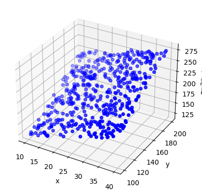
fig=plt.figure(num="Scatter")
ax1=plt.axes(projection='3d')
x=np.random.uniform(10,40,500)
y=np.random.uniform(100,200,500)
z=2*x+y
ax1.scatter(x,y,z,c="b")
ax1.set_xlabel("x")
ax1.set_ylabel("y")
ax1.set_zlabel("z=2*x+y")
plt.show()

结果如下：

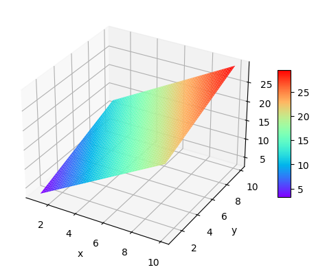
2.绘制平面图

#生成网格点矩阵坐标
x=np.arange(1,10,0.1)
y=np.arange(1,10,0.1)
X,Y=np.meshgrid(x,y)
Z=2*X+Y
#绘制平面
fig=plt.figure(num="Suface")
ax2=plt.axes(projection='3d')
surf=ax2.plot_surface(X,Y,Z,cmap="rainbow")
ax2.set_xlabel("x")
ax2.set_ylabel("y")
ax2.set_zlabel("z=2*x+y")
fig.colorbar(surf,shrink=0.5,aspect=10)#绘制颜色指示条
plt.show()

结果如下：

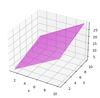
3.绘制线框图

#生成网格点矩阵坐标
x=np.arange(1,10,0.1)
y=np.arange(1,10,0.1)
X,Y=np.meshgrid(x,y)
Z=2*X+Y
#绘制线框图
fig=plt.figure(num="wireframe")
ax3=plt.axes(projection='3d')
ax3.plot_wireframe(X,Y,Z,color="m",linewidth=0.5)
ax3.set_xlabel("x")
ax3.set_ylabel("y")
ax3.set_zlabel("z=2*x+y")
plt.show()

结果如下：

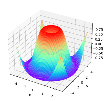
4.绘制曲面图

#生成网格点矩阵坐标
x=np.arange(-5,5,0.1)
y=np.arange(-5,5,0.1)
X,Y=np.meshgrid(x,y)
Z=np.sin(np.sqrt(X**2+Y**2))
#绘制曲面图
fig=plt.figure(num="曲面图")
ax4=plt.axes(projection='3d')
ax4.plot_surface(X,Y,Z,cmap="rainbow")
ax4.set_xlabel("x")
ax4.set_ylabel("y")
plt.show()

结果如下：

梯度下降法实现线性回归

1.NumPy实现

一元线性回归
- 加载样本数据x、y
- 设置超参数学习率、迭代次数
- 设置模型参数初值w0、b0
- 训练模型w、b
- 结果可视化

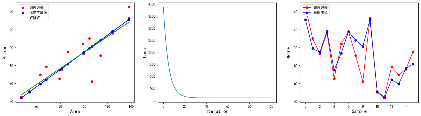
import numpy as np
import matplotlib.pyplot as plt
%matplotlib inline
#加载样本数据：x、y
x=np.array([137.97,104.50,100.00,124.32,79.20,99.00,124.00,114.00,106.69,138.05,53.75,46.91,68.00,63.02,81.26,86.21])
y=np.array([145.00,110.00,93.00,116.00,65.32,104.00,118.00,91.00,62.00,133.00,51.00,45.00,78.50,69.65,75.69,95.30])
#设置超参数学习率与迭代次数
learn_rate=0.00001
iter=100
display_step=10 #设置每十次迭代输出一次结果
#设置模型参数初值w0,b0
np.random.seed(612)
w=np.random.randn()
b=np.random.randn()
#训练模型w,b
mse=[]#用于记录每次的均方误差值
for i in range(0,iter+1):
    dL_dw=np.mean(x*(w*x+b-y))
    dL_db=np.mean(w*x+b-y)
    w=w-learn_rate*dL_dw
    b=b-learn_rate*dL_db
    #记录模型的预测值
    pred=w*x+b
    #计算并保存均方误差
    Loss=np.mean(np.square(y-pred))/2
    mse.append(Loss)
    #每十次迭代输出一次结果
    if i % display_step==0:
        print("i:%i, Loss:%f, w:%f, b:%f" %(i,mse[i],w,b))
#结果可视化
plt.figure(figsize=(20,5))
plt.rcParams["font.sans-serif"]="SimHei"
plt.rcParams["axes.unicode_minus"]=False

plt.subplot(1,3,1)
plt.scatter(x,y,color="red",label="销售记录")
plt.scatter(x,pred,color="blue",label="梯度下降法")
plt.plot(x,pred,color="blue")
plt.plot(x,0.89*x+5.41,color="green",label="解析解")
plt.xlabel("Area",fontsize=14)
plt.ylabel("Price",fontsize=14)
plt.legend(loc="upper left")

plt.subplot(1,3,2)
plt.plot(mse)
plt.xlabel("Iteration",fontsize=14)
plt.ylabel("Loss",fontsize=14)

plt.subplot(1,3,3)
plt.plot(y,color="red",marker="o",label="销售记录")
plt.plot(pred,color="blue",marker="o",label="预测房价")
plt.xlabel("Sample",fontsize=14)
plt.ylabel("PRICE",fontsize=14)
plt.legend(loc="upper left")

plt.show()

结果如下：

i:0, Loss:3874.243711, w:0.082565, b:-1.161967
i:10, Loss:562.072704, w:0.648552, b:-1.156446
i:20, Loss:148.244254, w:0.848612, b:-1.154462
i:30, Loss:96.539782, w:0.919327, b:-1.153728
i:40, Loss:90.079712, w:0.944323, b:-1.153435
i:50, Loss:89.272557, w:0.953157, b:-1.153299
i:60, Loss:89.171687, w:0.956280, b:-1.153217
i:70, Loss:89.159061, w:0.957383, b:-1.153156
i:80, Loss:89.157460, w:0.957773, b:-1.153101
i:90, Loss:89.157238, w:0.957910, b:-1.153048
i:100, Loss:89.157187, w:0.957959, b:-1.152997

多元线性回归
- 加载数据样本
- 数据处理：归一化、堆叠
- 设置超参数：学习率、迭代次数
- 设置模型参数的初值Wo
- 训练模型W：
- 结果可视化

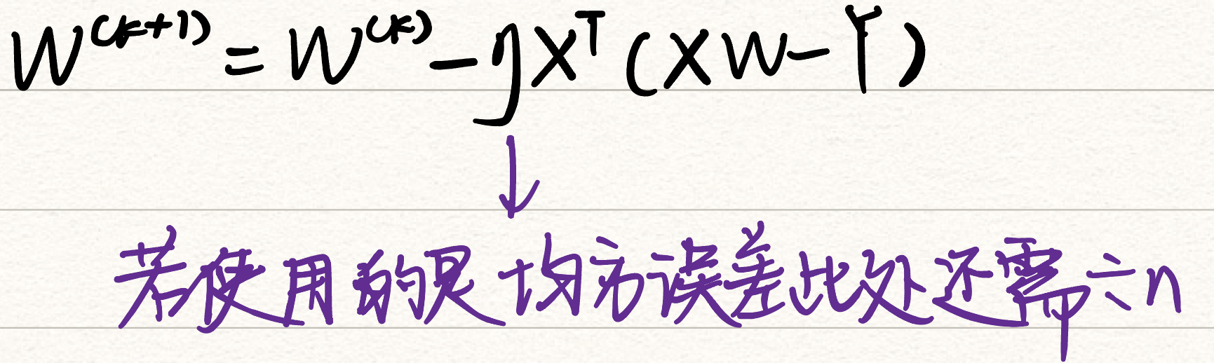
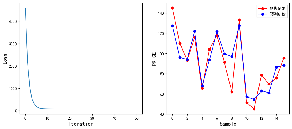
import tensorflow as tf
import numpy as np
import matplotlib.pyplot as plt
#加载样本数据
area=np.array([137.97,104.50,100.00,124.32,79.20,99.00,124.00,114.00,106.69,138.05,53.75,46.91,68.00,63.02,81.26,86.21])
room=np.array([3,2,2,3,1,2,3,2,2,3,1,1,1,1,2,2])
price=np.array([145.00,110.00,93.00,116.00,65.32,104.00,118.00,91.00,62.00,133.00,51.00,45.00,78.50,69.65,75.69,95.30])
num=len(area)#样本数量
#数据处理：归一化、堆叠
x0=np.ones(num)
x1=(area-area.min())/(area.max()-area.min())
x2=(room-room.min())/(room.max()-room.min())
X=np.stack((x0,x1,x2),axis=1)
Y=price.reshape(-1,1)
#设置超参数：学习率与迭代次数
learn_rate=0.2
iter=50
display_step=10 #设置每十次迭代输出一次结果
#设置模型参数初值W
np.random.seed(612)
W=np.random.randn(3,1)
#训练模型
mse=[]
for i in range(0,iter+1):
    PRED=np.matmul(X,W)
    Loss=np.mean(np.square(Y-PRED))/2
    mse.append(Loss)
    dL_dW=np.matmul(np.transpose(X),np.matmul(X,W)-Y)/num
    W=W-learn_rate*dL_dW
    if i % display_step==0:
        print("i: %i, Loss:%f" % (i,mse[i]))
#结果可视化
plt.figure(figsize=(12,5))
plt.rcParams["font.sans-serif"]="SimHei"
plt.rcParams["axes.unicode_minus"]=False

plt.subplot(1,2,1)
plt.plot(mse)
plt.xlabel("Iteration",fontsize=14)
plt.ylabel("Loss",fontsize=14)

plt.subplot(1,2,2)
PRED=PRED.reshape(-1)
plt.plot(price,color="red",marker="o",label="销售记录")
plt.plot(PRED,color="blue",marker="o",label="预测房价")
plt.xlabel("Sample",fontsize=14)
plt.ylabel("PRICE",fontsize=14)
plt.legend(loc="upper right")

plt.show()

结果如下：

i: 0, Loss:4593.851656
i: 10, Loss:85.480869
i: 20, Loss:82.080953
i: 30, Loss:81.408948
i: 40, Loss:81.025841
i: 50, Loss:80.803450

2.TensorFlow实现

一元线性回归

import tensorflow as tf
import numpy as np
#加载样本数据：x、y
x=np.array([137.97,104.50,100.00,124.32,79.20,99.00,124.00,114.00,106.69,138.05,53.75,46.91,68.00,63.02,81.26,86.21])
y=np.array([145.00,110.00,93.00,116.00,65.32,104.00,118.00,91.00,62.00,133.00,51.00,45.00,78.50,69.65,75.69,95.30])
#设置超参数学习率与迭代次数
learn_rate=0.0001
iter=10
display_step=1 #设置每一次迭代输出一次结果
#设置模型参数初值w0,b0
np.random.seed(612)
w=tf.Variable(np.random.randn())
b=tf.Variable(np.random.randn())
#训练模型w,b
mse=[]#用于记录每次的均方误差值
for i in range(0,iter+1):
    with tf.GradientTape() as tape:
        pred=w*x+b
        Loss=0.5*tf.reduce_mean(tf.square(y-pred))
    mse.append(Loss)
    dL_dw,dL_db=tape.gradient(Loss,[w,b])
    w.assign_sub(learn_rate*dL_dw)
    b.assign_sub(learn_rate*dL_db)
    if i % display_step==0:
        print("i: %i,Loss: %f, w: %f, b: %f" % (i,Loss,w.numpy(),b.numpy()))

结果如下：

i: 0,Loss: 4749.362305, w: 0.946047, b: -1.153577
i: 1,Loss: 89.861862, w: 0.957843, b: -1.153412
i: 2,Loss: 89.157501, w: 0.957987, b: -1.153359
i: 3,Loss: 89.157379, w: 0.957988, b: -1.153308
i: 4,Loss: 89.157364, w: 0.957988, b: -1.153257
i: 5,Loss: 89.157318, w: 0.957987, b: -1.153206
i: 6,Loss: 89.157280, w: 0.957987, b: -1.153155
i: 7,Loss: 89.157265, w: 0.957986, b: -1.153104
i: 8,Loss: 89.157219, w: 0.957986, b: -1.153052
i: 9,Loss: 89.157211, w: 0.957985, b: -1.153001
i: 10,Loss: 89.157196, w: 0.957985, b: -1.152950

多元线性回归

import numpy as np
#加载样本数据
area=np.array([137.97,104.50,100.00,124.32,79.20,99.00,124.00,114.00,106.69,138.05,53.75,46.91,68.00,63.02,81.26,86.21])
room=np.array([3,2,2,3,1,2,3,2,2,3,1,1,1,1,2,2])
price=np.array([145.00,110.00,93.00,116.00,65.32,104.00,118.00,91.00,62.00,133.00,51.00,45.00,78.50,69.65,75.69,95.30])
num=len(area)#样本数量
#数据处理：归一化、堆叠
x0=np.ones(num)
x1=(area-area.min())/(area.max()-area.min())
x2=(room-room.min())/(room.max()-room.min())
X=np.stack((x0,x1,x2),axis=1)
Y=price.reshape(-1,1)
#设置超参数：学习率与迭代次数
learn_rate=0.2
iter=50
display_step=10 #设置每十次迭代输出一次结果
#设置模型参数初值W
np.random.seed(612)
W=tf.Variable(np.random.randn(3,1))
#训练模型
mse=[]#用于记录每次的均方误差值
for i in range(0,iter+1):
    with tf.GradientTape() as tape:
        PRED=tf.matmul(X,W)
        Loss=0.5*tf.reduce_mean(tf.square(Y-PRED))
    mse.append(Loss)
    dL_dW=tape.gradient(Loss,W)
    W.assign_sub(learn_rate*dL_dW)
    if i % display_step==0:
        print("i: %i, Loss: %f" % (i,Loss))

结果如下：

i: 0, Loss: 4593.851656
i: 10, Loss: 85.480869
i: 20, Loss: 82.080953
i: 30, Loss: 81.408948
i: 40, Loss: 81.025841
i: 50, Loss: 80.803450

TensorFlow的可训练变量和自动求导机制

1.Variable对象

tf.Variable(initial_value,dtype)#initial_value可以是数字、Python列表、ndarray对象、Tensor对象
可训练变量赋值：
- 对象名.assign()
- 对象名.assign_add()
- 对象名.assign_sub()

#Variable对象：是可以被训练的变量，在模型训练过程中自动记录梯度信息，由算法自动优化
#创建
x=tf.Variable([[1,2,3,4],[4,5,6,7]])
print(x)
#trainalbe属性
print(x.trainable)
#对可训练变量赋值
print(x.assign([[1,2,3,4],[4,5,6,7]]))
print(x.assign_add([[3,2,4,5],[3,7,8,1]]))
print(x.assign_sub([[3,2,4,5],[3,7,8,1]]))#由结果可知，此操作改变了x对象本身

结果如下：

<tf.Variable 'Variable:0' shape=(2, 4) dtype=int32, numpy=
array([[1, 2, 3, 4],
       [4, 5, 6, 7]])>
True
<tf.Variable 'UnreadVariable' shape=(2, 4) dtype=int32, numpy=
array([[1, 2, 3, 4],
       [4, 5, 6, 7]])>
<tf.Variable 'UnreadVariable' shape=(2, 4) dtype=int32, numpy=
array([[ 4,  4,  7,  9],
       [ 7, 12, 14,  8]])>
<tf.Variable 'UnreadVariable' shape=(2, 4) dtype=int32, numpy=
array([[1, 2, 3, 4],
       [4, 5, 6, 7]])>

2.自动求导机制

GradientTape()的基本使用

#GradientTape()
#基本使用
x=tf.Variable(3.0) #必须是浮点数
with tf.GradientTape() as tape:
    y=tf.square(x)
dy_dx=tape.gradient(y,x)#dy_dx代表y对x的求导
print(y)
print(dy_dx)

结果如下：

tf.Tensor([9.], shape=(1,), dtype=float32)
tf.Tensor([6.], shape=(1,), dtype=float32)

GradientTape()的persistent参数

#当对多个函数同时求导时，需要将persistent=True,否则会报错因为其默认只计算一次求导，将其赋值为True后，需用del tape释放
x=tf.Variable(3.0) #必须是浮点数
with tf.GradientTape(persistent=True) as tape:
    y=tf.square(x)
    z=tf.pow(x,3)
dy_dx=tape.gradient(y,x)#dy_dx代表y对x的求导
dz_dx=tape.gradient(z,x)
print(y)
print(dy_dx)
print(40*"-")
print(z)
print(dz_dx)
del tape

结果如下：

tf.Tensor(9.0, shape=(), dtype=float32)
tf.Tensor(6.0, shape=(), dtype=float32)
----------------------------------------
tf.Tensor(27.0, shape=(), dtype=float32)
tf.Tensor(27.0, shape=(), dtype=float32)

GradientTape()的watch_accessed_variables参数

#默认watch_accessed_variables为True，表示自动监视可训练变量，若设置为False，则无法自动监视变量，可以使用watch()添加监视
x=tf.Variable(3.0)
with tf.GradientTape(watch_accessed_variables=False) as tape:
    tape.watch(x)#添加监视
    y=tf.square(x)
dy_dx=tape.gradient(y,x)#dy_dx代表y对x的求导
print(y)
print(dy_dx)

结果如下：

tf.Tensor(9.0, shape=(), dtype=float32)
tf.Tensor(6.0, shape=(), dtype=float32)

watch()添加监视

#watch()还可以监视非可训练变量
x=tf.constant(3.0)
with tf.GradientTape(watch_accessed_variables=False) as tape:
    tape.watch(x)#添加监视
    y=tf.square(x)
dy_dx=tape.gradient(y,x)#dy_dx代表y对x的求导
print(y)
print(dy_dx)

结果如下：

tf.Tensor(9.0, shape=(), dtype=float32)
tf.Tensor(6.0, shape=(), dtype=float32)

多元函数求偏导tape.gradient(函数，自变量)

#tape.gradient(函数，自变量)，这里的自变量可以是一个，也可以是多个，将多个自变量放在一个列表（元组）中，则可以对多元函数求偏导
x=tf.Variable(3.0)
y=tf.Variable(4.0)
with tf.GradientTape() as tape:
    f=tf.square(x)+2*tf.square(y)+1
df_dx,df_dy=tape.gradient(f,[x,y])
print(f)
print(df_dx)
print(df_dy)

结果如下：

tf.Tensor(42.0, shape=(), dtype=float32)
tf.Tensor(6.0, shape=(), dtype=float32)
tf.Tensor(16.0, shape=(), dtype=float32)

求二阶导数

x=tf.Variable(3.0)
y=tf.Variable(4.0)
with tf.GradientTape() as tape2:
    with tf.GradientTape() as tape1:
        f=tf.square(x)+2*tf.square(y)+1
    first_grads=tape1.gradient(f,[x,y])
second_grads=tape2.gradient(first_grads,[x,y])
print(f)
print(first_grads)
print(second_grads)

结果如下：

tf.Tensor(42.0, shape=(), dtype=float32)
[<tf.Tensor: shape=(), dtype=float32, numpy=6.0>, <tf.Tensor: shape=(), dtype=float32, numpy=16.0>]
[<tf.Tensor: shape=(), dtype=float32, numpy=2.0>, <tf.Tensor: shape=(), dtype=float32, numpy=4.0>]

对向量求偏导

x=tf.Variable([1.0,2.0,3.0])
y=tf.Variable([4.0,5.0,6.0])
with tf.GradientTape() as tape:
    f=tf.square(x)+2*tf.square(y)+1
df_dx,df_dy=tape.gradient(f,[x,y])
print(f)
print(df_dx)
print(df_dy)

结果如下：

tf.Tensor([34. 55. 82.], shape=(3,), dtype=float32)
tf.Tensor([2. 4. 6.], shape=(3,), dtype=float32)
tf.Tensor([16. 20. 24.], shape=(3,), dtype=float32)

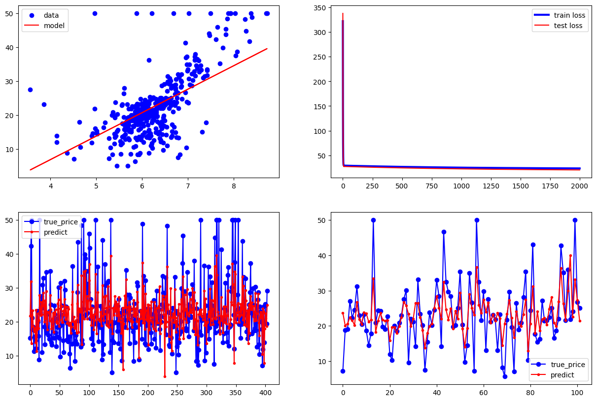
实例分析：波士顿房价预测

1.平均房间数与房价的关系

import tensorflow as tf
import numpy as np
import matplotlib.pyplot as plt
#加载数据集
boston_housing = tf.keras.datasets.boston_housing
#x表示房屋的属性值，y表示房价
(train_x,train_y),(test_x,test_y)=boston_housing.load_data()
x_train=train_x[:,5]
y_train=train_y
x_test=test_x[:,5]
y_test=test_y
#设置超参数：学习率与迭代次数
learn_rate=0.04
iter=2000
display_step=200 #设置每十次迭代输出一次结果
#设置模型参数初值w0,b0
np.random.seed(612)
w=tf.Variable(np.random.randn())
b=tf.Variable(np.random.randn())
#训练模型w,b
mse_train=[]#用来记录训练集上的损失（训练误差）
mse_test=[]#用来记录测试集上的损失（测试误差）
for i in range(0,iter+1):
    with tf.GradientTape() as tape:
        pred_train=w*x_train+b
        loss_train=0.5*tf.reduce_mean(tf.square(y_train-pred_train))
        pred_test=w*x_test+b
        loss_test=0.5*tf.reduce_mean(tf.square(y_test-pred_test))
    mse_train.append(loss_train)
    mse_test.append(loss_test)
    dL_dw,dL_db=tape.gradient(loss_train,[w,b])
    w.assign_sub(learn_rate*dL_dw)
    b.assign_sub(learn_rate*dL_db)
    if i % display_step==0:
        print("i:%i,\tTrain Loss:%f,\tTest Loss:%f" % (i,loss_train,loss_test))
#模型和数据可视化
plt.figure(figsize=(15,10))
plt.subplot(221)
plt.scatter(x_train,y_train,color="blue",label="data")
plt.plot(x_train,pred_train,color="red",label="model")
plt.legend(loc="upper left")
plt.subplot(222)
plt.plot(mse_train,color="blue",linewidth=3,label="train loss")
plt.plot(mse_test,color="red",linewidth=1.5,label="test loss")
plt.legend(loc="upper right")
plt.subplot(223)
plt.plot(y_train,color="blue",marker="o",label="true_price")
plt.plot(pred_train,color="red",marker=".",label="predict")
plt.legend()
plt.subplot(224)
plt.plot(y_test,color="blue",marker="o",label="true_price")
plt.plot(pred_test,color="red",marker=".",label="predict")
plt.legend()
plt.show()

结果如下：

i:0,    Train Loss:321.837585,    Test Loss:337.568634
i:200,    Train Loss:28.122616,    Test Loss:26.237764
i:400,    Train Loss:27.144739,    Test Loss:25.099327
i:600,    Train Loss:26.341949,    Test Loss:24.141077
i:800,    Train Loss:25.682899,    Test Loss:23.332979
i:1000,    Train Loss:25.141848,    Test Loss:22.650162
i:1200,    Train Loss:24.697670,    Test Loss:22.072006
i:1400,    Train Loss:24.333027,    Test Loss:21.581432
i:1600,    Train Loss:24.033667,    Test Loss:21.164261
i:1800,    Train Loss:23.787903,    Test Loss:20.808695
i:2000,    Train Loss:23.586145,    Test Loss:20.504938

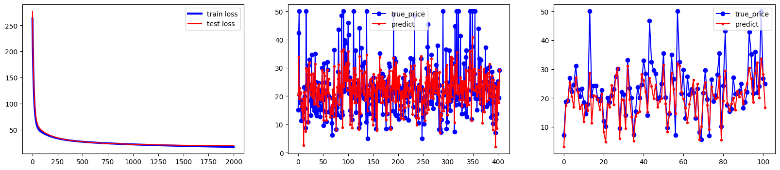
2.所有属性的多元线性回归

#加载数据集
boston_housing = tf.keras.datasets.boston_housing
#x表示房屋的属性值，y表示房价
(train_x,train_y),(test_x,test_y)=boston_housing.load_data()
num_train=len(train_x)
num_test=len(test_x)
#数据处理：归一化与拼接
x_train=(train_x-train_x.min(axis=0))/(train_x.max(axis=0)-train_x.min(axis=0))
y_train=train_y
x_test=(test_x-test_x.min(axis=0))/(test_x.max(axis=0)-test_x.min(axis=0))
y_test=test_y
x0_train=np.ones(num_train).reshape(-1,1)
x0_test=np.ones(num_test).reshape(-1,1)
X_train=tf.concat([x0_train,x_train],axis=1)
X_test=tf.concat([x0_test,x_test],axis=1)
Y_train=tf.constant(y_train.reshape(-1,1))
Y_test=tf.constant(y_test.reshape(-1,1))
#设置超参数：学习率与迭代次数
learn_rate=0.01
iter=2000
display_step=200 #设置每十次迭代输出一次结果
#设置模型参数初值W
np.random.seed(612)
W=tf.Variable(np.random.randn(14,1))
#训练模型W
mse_train=[]#用来记录训练集上的损失（训练误差）
mse_test=[]#用来记录测试集上的损失（测试误差）
for i in range(0,iter+1):
    with tf.GradientTape() as tape:
        PRED_train=tf.matmul(X_train,W)
        Loss_train=0.5*tf.reduce_mean(tf.square(Y_train-PRED_train))
        PRED_test=tf.matmul(X_test,W)
        Loss_test=0.5*tf.reduce_mean(tf.square(Y_test-PRED_test))
    mse_train.append(Loss_train)
    mse_test.append(Loss_test)
    dL_dW=tape.gradient(Loss_train,W)
    W.assign_sub(learn_rate*dL_dW)
    if i % display_step==0:
        print("i:%i,\tTrain Loss:%f,\tTest Loss:%f" % (i,Loss_train,Loss_test))
#模型和数据可视化
plt.figure(figsize=(20,4))
plt.subplot(131)
plt.plot(mse_train,color="blue",linewidth=3,label="train loss")
plt.plot(mse_test,color="red",linewidth=1.5,label="test loss")
plt.legend(loc="upper right")
plt.subplot(132)
plt.plot(Y_train,color="blue",marker="o",label="true_price")
plt.plot(PRED_train,color="red",marker=".",label="predict")
plt.legend()
plt.subplot(133)
plt.plot(Y_test,color="blue",marker="o",label="true_price")
plt.plot(PRED_test,color="red",marker=".",label="predict")
plt.legend()
plt.show()

结果如下：

i:0,    Train Loss:263.193459,    Test Loss:276.994119
i:200,    Train Loss:36.176548,    Test Loss:37.562946
i:400,    Train Loss:28.789464,    Test Loss:28.952521
i:600,    Train Loss:25.520702,    Test Loss:25.333921
i:800,    Train Loss:23.460534,    Test Loss:23.340539
i:1000,    Train Loss:21.887280,    Test Loss:22.039745
i:1200,    Train Loss:20.596287,    Test Loss:21.124848
i:1400,    Train Loss:19.510205,    Test Loss:20.467240
i:1600,    Train Loss:18.587010,    Test Loss:19.997707
i:1800,    Train Loss:17.797461,    Test Loss:19.671583
i:2000,    Train Loss:17.118926,    Test Loss:19.456854

ssy的小天地

TensorFlow实践之线性回归问题

解析法实现一元线性回归

1.纯Python实现

2.NumPy实现

3.TensorFlow实现

4.数据和模型可视化

解析法实现多元线性回归

三维模型可视化

1.绘制散点图

2.绘制平面图

3.绘制线框图

4.绘制曲面图

梯度下降法实现线性回归

1.NumPy实现

一元线性回归

多元线性回归

2.TensorFlow实现

一元线性回归

多元线性回归

TensorFlow的可训练变量和自动求导机制

1.Variable对象

2.自动求导机制

GradientTape()的基本使用

GradientTape()的persistent参数

GradientTape()的watch_accessed_variables参数

watch()添加监视

多元函数求偏导tape.gradient(函数，自变量)

求二阶导数

对向量求偏导

实例分析：波士顿房价预测

1.平均房间数与房价的关系

2.所有属性的多元线性回归